Analog simulation
The goal of analog simulation is to calculate a circuit's voltages and currents in accordance with Kirchoff's Current Law (KCL) and Kirchoff's Voltage Law (KVL). The following sections illustrate how the Analog Simulation Engine accomplishes this by discussing the core processes and core analysis modes.
There are three core processes which enable the simulator to solve analog circuits: Nodal Analysis, Linearization, and Numerical Integration.
Nodal Analysis is the most fundamental process and forms the basis for the Linearization and Numerical Integration processes.
Nodal analysis
Nodal analysis is the most fundamental process in the simulator. It is used to solve circuits with purely linear, non-differential elements, as shown below.
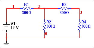
It is fundamental because more advanced circuit elements are always transformed into linear, non-differential form precisely so that this process can be used.
The Nodal Analysis process formulates a set of linear equations in accordance with Kirchhoff's Current Law (KCL) using a technique called Modified Nodal Analysis (MNA).
The simulator then uses matrix solving techniques to determine the solution to the set of linear equations. The process starts off with LU factorization. This involves decomposing the matrix A into two triangular matrices (a lower triangular matrix, L, and an upper triangular matrix, U) and solving the two matrices using forward substitution and backward substitution.
Several techniques are used to avoid numerical difficulties, to improve numerical calculation accuracy, and to maximize the solution efficiency. These include:
- A partial pivot algorithm that reduces the round-off error incurred by the LU factorization method.
- A preordering algorithm that improves the matrix condition.
- A reordering algorithm that minimizes nonzero terms for the equation solution.
Linearization
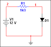
Non-linear elements pose a problem because the non-linear equations representing these elements cannot be solved directly as part of a system of equations. To address this problem, the simulator uses an iterative non-linear analysis technique called Newton-Raphson. To illustrate how this technique is used, consider the diode-resistor circuit shown below.
The exact analytical solution to the circuit is found at the intersection of the load line and the diode's I/V line, as shown below.
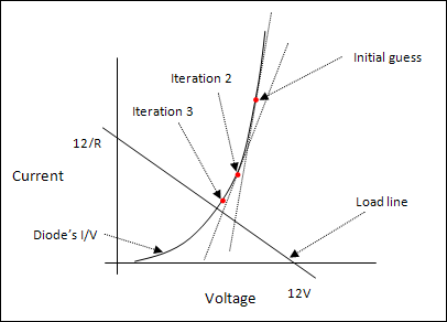
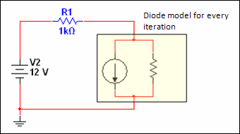
To find this intersection, the simulator begins by making a “guess” about the diode's voltage. The diode is then linearized about this guessed value using the derivative of the I/V curve. The linearization of the diode effectively models the diode as a resistor in parallel with a current source. This allows the simulator to use the Nodal analysis process to find a solution.
This first solution becomes the linearization value in the next iteration of the Newton-Raphson algorithm and the process continues until the difference in successive iterations becomes acceptably small. When this occurs, the iteration cycle is considered complete and the circuit solution is said to converge.
The example cited above is a very basic case of a non-linear circuit; the circuit contains only one non-linear element and there is continuity in the element's input-output curve and its derivative. In practice, the simulator has to deal with many non-linear elements and potential discontinuities in their input-output curves. As the number of non-linear elements increases, especially the number of elements with poor continuity characteristics, the chance for non-convergence likewise increases.
Convergence is one of the major hurdles in simulating non-linear circuits.
Convergence criteria
For every voltage node, the following must be satisfied:
|V1 - V2| < tol
where,
V1 is the value of the present iteration
V2 is the value of the previous iteration
tol is the tolerance defined as RELTOL * Max(|V1|, |V2|) + VNTOL
where RELTOL and VNTOL are simulator options.
For every voltage-defined branch (the branch contains either a voltage source or an inductor), the following must be satisfied:
|I1 - I2| < tol
where,
I1 is the value of the present iteration
I2 is the value of the previous iteration
tol is the tolerance defined as RELTOL * Max(|I1|, |I2|) + ABSTOL
where RELTOL and ABSTOL are simulator options.
Numerical integration
The numerical integration process is used in time-domain simulations (transient analysis). It is applied to elements with differential behavior. That is, their input/output relationship is of the form y = f(dx/dt), as found in a capacitor. These are called reactive elements.
Like non-linear elements, reactive elements pose a problem for finding a solution because the differential equations cannot be solved directly as part of a system of equations. To solve circuits with reactive elements, the simulator uses numerical integration methods. In numerical integration, the integral or derivative is approximated by discretizing it in accordance with some formula.
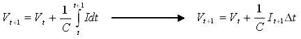
For instance, assume that we know the voltage of the capacitor at time t and would like to find the voltage at time t+ Δt. We can use the Backward Euler formula to discretize the integral into an algebraic expression, as shown below.
According to the formula above, at time t+1, the capacitor in the following circuit,
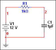
is discretized into the model shown in the following circuit.
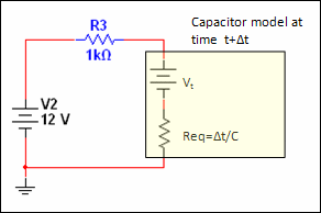
Like the diode, the capacitor becomes a composition of linear, non-differential elements and can therefore be solved using matrix solving techniques.
The Backward Euler method is used only for illustrative purposes. The Multisim simulator actually uses either the Trapezoidal or Gear Integration Methods, both of which have superior characteristics in terms of accuracy. (The Thevenin representation of the capacitor model is also used for illustrative purposes. During numerical integration, the simulator actually uses a Norton representation in which a current source is in parallel with a resistor).
Note that the discretized capacitor model is sensitized to the size of the time step, which is always proportional to the size of the error in approximating the integral.